Precision Timing in the Power Industry: How and Why We Use it

Time in the Power Industry: How and Why We Use It

Bill Dickerson, P. Eng. Arbiter Systems^®, Inc.

Introduction

Precise, reliable time is now available at reasonable cost to users worldwide. In the power industry, engineers have made use of precise time in numerous applications to:

• Improve reliability
• Reduce costs
• Better understand power system operation
• Predict and prevent system-wide faults
• Test and verify operation of protective devices

This paper will explain some of these applications, describe the requirements of the applications, provide information about sources and distribution of precise time, and help you to understand how to successfully apply commercially-available products to synchronize power system equipment.

Applications of Precise Time

The value of time synchronization is best seen by understanding that the power grid is a single, complex and interconnected system. What happens in one part of the grid affects operation elsewhere. Understanding, and possibly controlling, these interactions requires a means to compare what is happening at one place and time with that happening at other places and times. Precise time and high-speed communications in the substation are the enabling technologies which make this practical.

Event Reconstruction

When these complex interactions, usually in reaction to external stimuli, lead to major events such as cascading faults and large blackouts, recording devices installed at various points in the grid generate large numbers of reports and data files. Making sense of these files on a systemwide basis requires establishment of a common frame of reference. This consists of a spatial frame of reference; i.e. what happened where, as well as a temporal frame of reference, i.e. what happened when.

The spatial frame of reference comes directly from the network topology, which is generally well known to the engineers involved. Without some sort of accurate time mark in the data files, however, establishing the temporal frame of reference is challenging at best, and may be impossible. And, where possible, it often requires a great deal of effort. Indeed, in the analysis of the large blackout of August 14, 2003 affecting much of eastern North America, more time was spent ordering and manually time-tagging unsynchronized event recordings than on any other task.

This is done by looking for common, recognizable characteristics in the data files, usually by plotting them and visually inspecting the printouts. If one of the files has an accurate time tag, then the other may be ‘tagged’ by inference. As the events get more complex, with more and more ‘noise’ from other things happening at the same time, this becomes more difficult and eventually, impossible. And, as the ‘degrees of separation’ from each record to one with an accurate time-tag increases, the expected accuracy of the time frame of that record gets worse.

Synchrophasors

Synchrophasors are “synchronized phasor measurements,” that is, measurements of ac sinusoidal quantities, synchronized in time, and expressed as phasors. With a fixed temporal reference frame, synchrophasor measurements may be used to determine useful information about operation of the grid.

For example, power flows may be monitored in real-time, and by measuring changes in the phase shift across parts of the grid, estimates of stress and future stability can be made. Postprocessing of synchrophasor data (which can also be done in real time) can extract information about low-frequency system modes, and by examining whether the amplitudes of these modes are changing, advance warning of impending instability can be given.

Synchrophasor measurements are made practical by a widespread, economical source of accurate time.

System Time and Frequency Deviation

One of the oldest and most widespread uses of accurate substation time is monitoring the average system frequency. While the grid itself, and the machines connected to it, generally have a reasonable tolerance so far as small frequency offsets is concerned, many customers use the line frequency as a sort of time standard. Consider how many clocks in your own home require resetting when the power fails, even briefly.

All of these devices use the line frequency as their time standard. The short-term frequency is less important for this sort of timekeeping than the frequency averaged over a period of hours or days. This allows the utility to control frequency during times of peak load, as one of many variables to direct power flows and ensure orderly operation of the grid. Then, when load is down (generally in the early morning hours), the frequency can be adjusted to “zero out” the accumulated time offset. System time and frequency monitors provide the information required to do this, by measuring and comparing system time (from the grid frequency) to precise time.

Multi-Rate Billing

Eager to improve overall system utilization, utilities offer certain customers incentives to use power at off-peak hours by providing them with lower energy rates during these periods. While this seems simple enough, the amounts of money can be considerable, and a meter with a simple real-time clock that slowly drifts off (until it is reset) probably will not be acceptable as a basis for determining billing periods.

Today, the cost to provide accurate time, directly traceable to national standards, is quite reasonable. It is practical to provide an accurate clock right at the customer premises, connected directly to (or part of) the revenue meter.

Power Quality Incentives

Utilities and system operators are now considering, and in some cases implementing, financial incentives to customers to maintain power quality. Certain types of load are well-known for causing power quality impairments, such as harmonics and flicker.

These power quality impairments are measured in accordance with international standards, such as the IEC 61000-4 series. Harmonics and flicker are summarized in reporting periods, generally 10 minutes (though other periods can be used). As with multi-rate billing, the amounts of money can be significant, so customers often operate their own monitor ‘in parallel’ with that of the utility. Nothing causes disputes faster than monitors that disagree on the measurements, and the measurements are certain to disagree if the reporting periods are not synchronized.

Providing accurate, traceable time eliminates this potential source of disagreement. Low-cost, accurate clocks are therefore an enabling technology for power quality incentives.

Time Tagging Recorded Data

Many power industry standards allow data to be stored or transmitted with an associated time tag. Examples include IEEE C37.111, COMTRADE, for file storage; and IEC 61850 for substation communications. Presumably, these time tags can be used to aid in comparing data from different sources when reconstructing a power system event, or when merging data from multiple sources into one data stream.

However, these standards do not typically specify how time tags are to be determined. Time tags might be generated at the time the data is sampled; at the time an event is recognized; or at the time a message or record is processed by a software communications protocol stack. Lack of consistent and accurate time tags in the data files generated during large power system events has made blackout and event analysis more difficult and time consuming.

The only meaningful definition for a time tag (with respect to later use of the information) requires that the time tag match the actual time of occurrence of an event, or the actual time that a power system quantity was equal to its reported value, within stated uncertainty limits. In practice, this definition has rarely been observed. IEEE’s Power System Relaying Committee of the Power Engineering Society (PES-PSRC) has convened a Working Group (H3) to address this issue.

Remedial Action Schemes / Wide Area Measurement Systems

Remedial action schemes (RAS), based on wide-area measurement systems (WAMS), are being developed with the goal of enabling system-wide protective actions to be taken in power systems. By detecting impending instabilities in the grid, ‘remedial actions’ such as dropping load or generation, adjustment of VAR compensation, or dynamic braking, can be initiated to attempt to control the instability and prevent it from developing into a full-scale event, such as a cascading failure.

Monitoring and controlling the grid in this way requires a ‘big-picture’ view. Local operators are normally unaware of conditions leading up to a cascading failure caused by overall system instability, until the system begins to break up and assets start dropping off-line due to local protection operation.

RAS/WAMS require synchronized measurements of power system quantities, such as frequency, voltage, active and reactive power flows, and phase angle differences. These measurements are often made with Phasor Measurement Units (PMUs) but can also be made using other synchronized measuring devices.

Traveling-Wave Fault Detection

Faults in transmission lines often occur in remote locations, and repairing them can be time consuming, especially if the location of the fault is unknown. Traveling-wave fault location is a method of estimating the location of a fault based on measuring the difference in arrival times of fault artifacts at the two ends of a faulted line.

Most faults generate a waveform containing a significant amount of high-frequency energy.This can be caused by the primary event initiating the fault, such as a lightning strike or tree hit and the resulting arc; or it can be caused by a break in the line due, for example, to snow, ice, and/or wind loading. This high-frequency energy can often be detected with excellent resolution in the time domain. This event ‘signature’ propagates down the transmission line at nearly the speed of light. Therefore, the ‘signature’ will be received at the ends of the line at times equal to the time of the fault event, plus the propagation delay along the line. If the arrival times at both ends of the line can be measured, then the location of the fault can be estimated. With a good fault signature and accurate time, the fault can be localized to the nearest transmission tower, expediting dispatch of repair crews.

End-to-End Relay Testing

Many protection schemes require the proper coordination of relay settings at the two ends of a transmission line. These settings are determined by engineers using models of the power system. Verification of proper operation is performed using two relay test sets, each connected to a relay at the two ends of the line. These test sets must be synchronized, so that they can generate fault waveforms with the proper time relationship at the two ends of the line. These signals are presented to the relays, and proper operation of the relays and communications network can be verified.

Accuracy Requirements

Event Reconstruction with Recorded Data

Event reconstruction generally requires that records can be re-aligned within a fraction of a power line cycle. At 60 Hz, a power line cycle is 16.7 ms; at 50 Hz, 20 ms. Successful reconstruction is possible with time tags delivering an accuracy of about a quarter of a cycle (4 ms to 5 ms) but better accuracy usually makes the job easier. NERC standard PRC-018-0 requires that the clock in a substation Disturbance Measuring Equipment (DME) be set to an accuracy of 1 ms, which (allowing for other errors in the DME) will generally allow overall time accuracy in the recorded data file of less than 2 ms. Commonly, 1 ms has been considered the goal for synchronizing DME devices such as sequence of event recorders, digital fault recorders, and relays with event recording functions.

Phasor Measurements, RAS/WAMS

Synchrophasor measurements, compliant with IEEE Standard C37.118, must not be in error by more than 1 % ‘total vector error’ (TVE), where this error includes components due to time offsets in the PMU clock; phase errors or delays in the signal processing circuitry; and magnitude errors. 1 % TVE corresponds to a phase angle error of 0.57 degrees, if no other errors are present. This is about 26 microseconds at 60 Hz (32 µs at 50 Hz).

If we allow time synchronization error to be 20 % of the error budget, this allows for a time error in the PMU of 5 µs to 6 µs. This level of error is easily met with current technology. However, realistically, in a typical substation errors in the instrument transformers often contribute a few degrees of phase shift, especially with relaying CTs operating at nominal (non-fault) current levels. Under realistic conditions, therefore, even an error of several tens of microseconds is unlikely to have much effect on the measurement.

System Time and Frequency

Time offsets have no effect on frequency measurements, provided that the time offset is constant. This is because frequency is the rate of change of phase (time); so any fixed phase or time error will cause zero frequency error.

Time offsets will cause an error in the system time measurement, which again is an estimate of the time indicated by a synchronous-motor clock attached to the power line. Allowable error is therefore a direct function of the accuracy required in measuring system time. Since the application relates to timekeeping with mechanical clocks for human activities, an error of a fraction of a second is likely to be acceptable. If we consider also using the power line as a time base for automated timekeeping, the error requirements tighten to a few milliseconds.

Billing and Power Quality Incentives

Keeping accurate time is necessary for this application since fair performance of contract requirements requires the utility (and customer, if applicable) to apply the correct rates for the proper intervals of time. Often, these incentives are coupled with the customer’s efforts to move load to off-peak periods.

The accuracy required ranges from a fraction of a second, for basic billing considerations, to perhaps as little as a millisecond where the clock is used to synchronize periodic measurements of power-quality quantities such as harmonics and flicker. Different measurement intervals will yield different results, possibly leading to conflict between utility and customer.

Traveling-Wave Fault Detection

Because fault waveforms travel at the speed of light, or very nearly, this application imposes the most stringent requirements of all those listed. If, for example, towers are located 500 meters apart, and the goal is to locate a fault to the nearest tower, then the maximum time error which can be tolerated (between the two clocks at the ends of the line) is the amount of time it requires the signal to travel 500 meters. At the speed of light, this is about 1.7 µs.

Since there are also other sources of error, it is best to keep the error well below this. GPS and other precise sources of time can provide accuracy of 100 nanoseconds (0.1 µs) or better, so this requirement can be met, with proper care in application.

End-to-End Relay Testing

This is another application that requires fraction of a power line cycle accuracy. Relays generally operate on a cycle-by-cycle basis, so an accuracy of one millisecond is typically adequate. Better accuracy is possible, further reducing time errors as a problem in this application.

Time Scales, Time Zones Etc.

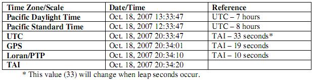
Time Scales: UTC, TAI, GPS, LORAN…

The international timing community, headquartered at the International Bureau of Weights and Measures in Paris (known by the acronym of its French name, BIPM) maintains the International Atomic Time scale (again in French, TAI). This time is maintained by what is, in effect, an ensemble of hundreds of atomic clocks around the world, owned and maintained by the national standards laboratories that are members of BIPM. These include NIST and USNO in the USA, NRC in Canada, CSIRO in Australia, and the Royal Observatory in England.

Because of variations in the rotation of the Earth, TAI has drifted away from astronomical time. It is presently about 33 seconds ahead, since the rotation of the Earth is somewhat slower than it used to be.

‘Civil time,’ which is used by most government, commercial, and private users, is corrected for this difference. This time scale is called ‘UTC’ or Coordinated Universal Time. UTC is offset from TAI by an integer number of seconds. This keeps it within a second of astronomical time, which is adequate for most applications.

Precise navigation applications which need better accuracy may use the time scale ‘UT0’ which incorporates fractional second corrections to UTC.

Other time scales, for example the LORAN time scale used by the ‘Long-Range Aid to Navigation’ system, are generally related to TAI or sometimes UTC. LORAN time, for example, is equal to TAI – 10 seconds and GPS time is equal to TAI – 19 seconds. These differences come about because these time scales were once equal to UTC, when their ‘epoch’ began; but they have drifted from UTC as UTC has been adjusted to follow astronomical time.

Examples of time zones and scales for the same second:

What Is GMT?

GMT stands for ‘Greenwich Mean Time.’ GMT was formerly (prior to UTC) the de-facto world standard for civil time, maintained by the Royal Observatory at Greenwich, England. It followed the mean solar day at the Greenwich Meridian.

GMT is now obsolete, having been replaced January 1, 1972 by UTC. The term GMT is still used (incorrectly, but commonly) for one of two purposes:

• As an alternate name for the UTC time scale;
• As an alternate name for Western European (winter) Time zone (WET).

Time Zones and Local Time

Most locations around the world do not use UTC directly but rather use a version of UTC adjusted so that local civil time is approximately the same as local solar time, i.e. the sun is approximately overhead at noon. ‘Time zones’ are areas that use a common format of local time. In most cases, time zones use an offset that is an integer number of hours different than UTC. For example, California is in the Pacific Time Zone, and Pacific Standard Time is eight hours behind UTC.

Some locations use time zones that differ by something other than an integer number of hours. India and parts of Australia and Canada are examples.

Daylight Savings or Summer Time

Many parts of the world change their time zone offset during local summer. This shift is generally by one hour, and it is designed to make the period of usable daylight, after suppertime, longer by an hour.

Legislative Issues for Local Time

Both the time zone to use, and the definition of summer time, are creations of man and subject to frequent changes. Recently, for example, the definition of daylight savings time in the USA was changed. Most provinces of Canada (after grumbling) followed the US lead.

Some states in the USA, for example Arizona, do not observe daylight savings time at all. In other states, some counties do and some do not.

Because of these issues, users of local time must always be prepared to adjust their timekeeping accordingly, or risk being ‘out of step’ with those around them.

Leap Seconds

Leap seconds are used to adjust the difference between TAI (which is a continuous, monotonic time scale) and UTC (which is not), to keep UTC approximately the same as astronomical or solar time. A leap second is an ‘extra second’ added to compensate for the slowing of the Earth’s rotation. Negative leap seconds can happen if the Earth’s rotation were to increase in speed. However, that is not likely since the tides and other drag mechanisms are expected to continue to slow the rotation.

Leap seconds are introduced, by convention, at midnight UTC at the end of a month. Generally, leap seconds are introduced in the months of June or December though they can happen any month. Keep in mind that (due to local time zone offsets) the leap second will happen at a different time than midnight, in time zones other than Western European Time. The time sequence during a normal (added) leap second looks like this (for UTC and Pacific Standard and Daylight Time Zones):

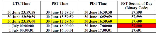
Note that the introduced leap second (in yellow), with a seconds value of 60, will not be accepted by many systems as a valid time. Also notice that the binary seconds value of two successive seconds can be the same (red). Both of these issues cause problems for real-time systems.

There has been a discussion towards eliminating leap seconds in civil time (UTC). Telecom network operators, for example, are in favor; astronomers are opposed. Remember that civil time was once kept by astronomers, who therefore view UTC as ‘their’ time. Time will tell whether this effort to eliminate leap seconds will be successful or not.

Coordinating Time Across a Network or Power Grid

The multitude of local time zones, periodic actions by legislators to redefine local time, and inconsistent application of summer time across jurisdictions lead to complications when comparing data from sources spread across a large geographical area. Accordingly, NERC requirements are forcing utilities to convert to UTC for data stored in event files, or transmitted across data networks. This eliminates uncertainty caused by local time issues.

Note that local operators can still view data in local time. Visualization programs include (or will soon include) the ability to convert records stored in UTC to local time.

Arbiter has recommended using UTC for these purposes for many years, and concurs with the NERC recommendations.

Sources of Precise Time

Global Navigation Satellite Systems (GNSS)

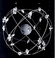
Global navigation satellite systems, of which GPS is the best-known example, are worldwide satellite navigational systems which maintain a constellation of satellites in orbit around Earth, whose signals may be received to determine precise position and time anywhere. Finding position (3 variables, X, Y and Z) and time (T) requires measurements from at least four satellites, so these systems generally try to guarantee that more than four are visible at all times, everywhere on Earth.

Accuracy is typically less than 50 meters for position and less than 100 nanoseconds in time, when receiving a minimum of four satellites.

Note that if the position is known (after the receiver has seen four satellites and is in a fixed position, or if it can be given a surveyed position), only one satellite is required thereafter to maintain accurate time. If more than one satellite is visible, time from each may be averaged, resulting in reduced error in the time estimate.

GPS’s large lead in deployment, and the free availability of its basic signals, has given it a near monopoly on end-user or ‘terminal’ equipment. GPS receivers are manufactured in large volumes as consumer commodities, which has driven the price to the point where the economic attractiveness of alternatives has been reduced. However, there do exist some systems (though not for timing) which can receive signals from multiple systems, most commonly GPS and GLONASS. Over time, receivers (including timing) will probably be made available for the other GNSS. If past patterns are an indicator, this will likely start with high-end equipment used, for example, by national laboratories for test and comparison purposes.

GPS

The Global Positioning System was the first GNSS, developed and operated by the United States Department of Defense, and was originally called NAVSTAR. This system was put into operation, in a development mode, in the 1980s and became fully operational in 1993. In addition to precise position anywhere in the world, the GPS system provides a free, civilian timing signal with accuracy that is now better than 10 nanoseconds.

The GPS system consists of at least 24 satellites (the ‘space segment’) and a set of receivers on the earth (the ‘control segment’). The satellites orbit the earth at approximately 20 200 km (12,600 miles) above the surface and make two complete orbits every 23 hours 56 minutes (a ‘sidereal’ or astronomical day). The GPS satellites

continuously broadcast signals that contain data on the satellite’s precise location and time. The satellites are equipped with atomic clocks that are precise to within a billionth of a second. The control segment continually monitors performance of the satellites and adjusts their internal clocks as required to maintain accuracy.

Usually GPS clocks provide a timing reference with an accuracy of one microsecond or better. In a power system with 60 Hz system frequency, one microsecond corresponds to 0.0216 degrees in 60 Hz phase angle (0.018 degrees at 50 Hz). Therefore, the timing reference provided by the GPS system is accurate enough for most power system applications.

The GPS operates on its own internal system time scale, GPS Time which is TAI-19 s. Correction factors are provided so that a GPS clock can provide UTC Time Scale.

The cost of the GPS system – estimated at over USD750 million per year – is paid by the US government, and the signals it provides are free to users worldwide.

GLONASS

The Russian GLONASS (Global Navigation Satellite System) provides similar capabilities to GPS. Sporadic funding of GLONASS and the resulting inconsistent satellite coverage have hampered widespread acceptance of the GLONASS system, although it is in some ways superior to GPS with respect to accuracy. Originally developed under the Soviet regime, GLONASS was allowed to degrade after the breakup of the Soviet Union. The Russian government has renewed its commitment to GLONASS, and recent launches have restored its operational capabilities.

Developing Systems: Galileo, Beidou

Other GNSS systems include the EU Galileo, and China’s Beidou (Compass). All work on a similar basis as GPS, and all are potentially capable of providing accurate world-wide time. Four experimental Beidou-1 satellites are on-orbit, but the operational Beidou-2 has not yet been deployed. While the Chinese government says the system will be operational in 2008, no Beidou-2 satellites have yet been built. China is also participating in the Galileo system.

Galileo is presently under development, and the first on-orbit test satellites (GIOVE) have been launched. Full operational capability is still many years away.

India is also developing a system, called IRNSS.

Standard Radio Transmissions

Radio stations such as WWV and WWVB in the USA, CHU in Canada, and DCF in Germany also provide standard time signals. They are not compensated for transmission delays, and those which operate in the HF bands are subject to ionospheric effects. These signals are also subject to severe interference due to corona noise generated in proximity to high-voltage equipment. Therefore, they have limited usefulness in a power system environment.

Microwave or Terrestrial Distribution

Some utilities have (in the past) built their own system to distribute time throughout their own network. Today, with the reliability and low cost of commercially-available GNSS timing receivers, these utilities are de-commissioning their internal timing systems.

Atomic Standards

Some utilities have also used atomic standards in the past. Cesium beam oscillators can keep very accurate time over a period of years, and by periodic comparison to national standards, can be adjusted to stay within the required performance limits over their useful life. However they are very expensive (USD60,000) and require periodic replacement of their cesium beam tube, at significant expense. Atomic standards have again been superceded by low-cost GPS receivers in utility applications.

Methods of Timing Distribution

Some substation Intelligent Electronic Devices (IED) include built-in GPS receivers to provide precise timing. More commonly, however, substations include numerous IEDs which all can benefit from synchronization. Therefore, utilities have generally opted for a satellite clock in the substation, which provides timing signals to the various IEDs. The following sections describe various methods that have been used for timing distribution, with varying levels of cost, complexity and performance.

Dedicated Timing Signals

Dedicated timing signals require a connection specifically for timing. Most equipment used in substations today (over 95 %) uses dedicated timing signals. 90+ % of these are IRIG-B.

1PPS

One pulse per second (1PPS) signals provide excellent accuracy (on-time mark), limited only by the care taken in the quality of the connection of the source to the device being synchronized. Better than 100 ns is routinely achievable. However, the 1PPS signal does not provide any indication of the date or time of day, so its use as a time code has been supplanted (for power applications) by the IRIG time codes which can provide equal accuracy and also provide time-of-year information.

1PPS is still commonly used in standards laboratories, to compare time and frequency sources at the highest level of accuracy.

IRIG Time Codes

The Inter-Range Instrumentation Group (IRIG) of the Range Commanders’ Council, a US military test range body, was faced several decades ago with a problem. Each test range had developed its own, unique time code. These time codes were recorded with test data on data tape recordings. The time codes were all incompatible, which made it difficult or impossible for the ranges to exchange data. Therefore, IRIG set about developing a common set of time codes. These have become known as the ‘IRIG codes.’

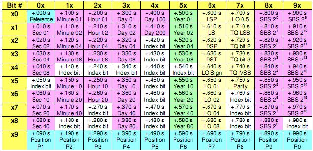
These time codes have become widely used in both military and civilian applications. Particularly, the IRIG code B (generally abbreviated IRIG-B) has become widely accepted for time distribution in substations. This time code repeats each second, and has a total of 100 bits per second. Some of these are framing (sync) bits, some are assigned for time, and some are available for control functions (tables 1 and 2). The basic IRIG-B code has an ‘ambiguity’ of one year, since it does not contain year data. The IRIG codes can provide both time-of-day information, and an accurate on-time mark.

IRIG-B code may be used in either logic-level (unmodulated) format, or as an amplitude modulated signal with a 1 kHz carrier (below). The modulated IRIG signal is particularly suitable for transmission over voice-band channels, including data channels on an instrumentation tape recorder. Because of the difficulty of accurately measuring the zero crossings, modulated IRIG-B code is capable of an accuracy better than one millisecond (one period of 1 kHz), but not usually better than ten microseconds. This level of accuracy is acceptable for some but not all substation applications. Modulated IRIG inputs to IEDs are generally transformer-isolated and provided with an automatic gain-control stage, so as to accept input signals with a wide range of amplitudes. A typical input level range is 0.1 Vpp to 10 Vpp.

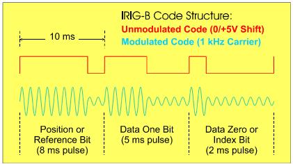
The unmodulated IRIGB code can deliver accuracy limited only by the slew rate of the digital signal, much better than one microsecond and, with care, in the range of a few nanoseconds. Unmodulated IRIG-B is normally distributed at a level of 5 volts (compatible with TTL or CMOS inputs). While some IEDs couple the IRIG-B signal directly to a logic gate, best practice has for some time used an optically-isolated input to break ground loops. Well designed substation clocks can generally drive numerous inputs with either modulated or unmodulated IRIG-B signals, so a single clock can synchronize all the IEDs in a substation.

{{The current version of the IRIG standard is IRIG Standard 200-04. It is available on the Arbiter Systems, Inc. web site.

IEEE-1344 Extension to IRIG-B Time Code

The IRIG codes were originally developed for test-range use, and a one-year ambiguity was acceptable. Being a military code, times were always recorded in UTC (Coordinated Universal Time, military Zulu Time), so local offsets and summer time issues were also not a concern. Leap seconds, which happen once or twice a year or less, also were not a concern of the IRIG group. And the range officer would be required to guarantee that all recorders were synchronized properly before beginning a test.

Real-time operation, 24 hours per day, 365 days per year, year after year, imposes some additional requirements. The issues identified in the previous paragraph become real concerns. As part of the original Synchrophasor standard, IEEE Standard 1344-1995, an extension for the IRIG-B code was developed using the ‘control bits’ field to provide an additional 2 digits of year (subsequently adopted also by the IRIG standard), as well as local offset, time quality, and bits for leap second and summer time changeovers. Some IEDs support this extension, but many do not. You may find an occasional IED that requires the IEEE-1344 extension for proper operation. This may not be well documented in the product literature.

The IEEE-1344 extension also created a new ‘modified Manchester’ encoding scheme, which is a digital signal having zero average value, and suitable for transmission over an optical fiber. It encodes the same 100 bit/second data stream onto a 1 kpps square-wave carrier. This modulation method has also been accepted as part of the IRIG standard.

Signal levels and connection methods for the IRIG-B code, with or without the IEEE-1344 extensions, are identical. The only difference is the use of the control bits to provide the extra information required in continuous, real-time monitoring applications (below). This is a firmware feature, and does not affect the hardware interface. IEEE Standard 1344 has been supplanted by IEEE Standard C37.118, which also includes this information. This standard may be purchased from the IEEE in New Jersey, USA

Serial (ASCII) Broadcast Time Codes

Many clocks provide a choice of ASCII strings, containing the time, which can be sent over a hardware serial port such as RS-422 or EIA-232. Generally, one of the characters in this string is transmitted ‘on time,’ more or less. One example of this sort of time code is IRIG Code J.

The accuracy in generating and receiving this sort of time code is a function of the hardware latency in the serial ports, usually a few bit times, plus firmware and/or software latency in the clock and client operating system. At higher bit rates, such as 19200 baud and higher, these errors can be kept below a millisecond.

This sort of time code is used quite often, primarily to drive large-digit time displays and to synchronize computers. Sometimes, the time data stream is interleaved with measurement data, for example, when the clock also provides the function of a system time and frequency monitor.

A few older IEDs were designed to accept this sort of synchronization, but this is becoming uncommon, since better methods are available. ASCII time codes can be used to resolve the ambiguity of a 1PPS signal, providing the on-time mark accuracy of 1PPS and the time-of-year from the serial time code. However, this practice requires two connections to the IED, and has largely been supplanted by IRIG-B.

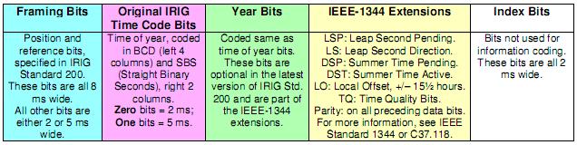
Network Time Synchronization

With the proliferation of IEDs in a modern substation, it is a natural question to ask: can we use the same connections to provide both data and synchronization? Within some limits, the answer is yes.

NTP and SNTP

NTP (Network Time Protocol) is a software method to transfer time between computers using a data network, such as the Internet. NTP is defined in an Internet Request for Comment document, RFC-1305. NTP generally provides moderate accuracy, from a few milliseconds up to a few hundred milliseconds depending on the nature of the connection between the NTP client and the server, and the performance of the computers’ operating systems. NTP includes methods to estimate the round-trip path delay between the server and client, and to ignore ‘outliers,’ or path delay estimates which vary significantly from the typical value. However, even in the best case of a local network (e.g. Ethernet), typical performance is limited by the operating system stack latency, and is often no better than one millisecond.

SNTP is a version of NTP that does not include the sophisticated clock-discipline algorithms included in NTP. SNTP may be used at the ‘roots’ or ‘leaves’ of a network: points where time is either first sent to the network (from an accurate source such as GPS), or received by a client (such as an IED). Since this topology is valid for many simple substation networks, SNTP can be used in both servers (GPS clocks) and clients (IEDs) in a substation, with no need for NTP.

For best accuracy, the logical connection between the server and client should be as short as possible. With optimum design of both server and client, and optimum configuration of the network, accuracy of a few microseconds is possible. Arbiter is now working toward making this level of performance practical in the substation environment.

It is a common misconception that SNTP is less accurate than NTP. Actually, so far as time transfer is concerned, they are the same. The clock discipline algorithms added in NTP are required for stability in large, complex networks (like the Internet) where NTP servers will be disciplined to several lower-stratum (more accurate) servers themselves, and in turn discipline potentially thousands of clients. In the ‘roots’ and ‘leaves’ of a network, these algorithms are not required and performance is the same. In simple networks that can be implemented using SNTP alone, accuracy far better than that typically associated with ‘regular’ NTP is possible.

NTP’s standard level of performance is adequate to resolve the one-second ambiguity of a 1 PPS signal, however, so NTP and 1 PPS together make an acceptable method of accurate time synchronization in a substation (right). This requires two connections to the IED, and so is not generally an optimal solution. We have seen in the discussion above how the dedicated logic-level input can be used alone to provide accurate time, using IRIG-B code. A natural question then is: can a network connection be used in some way to provide better time accuracy than NTP?

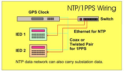
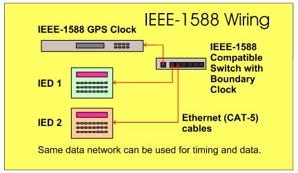
PTP (IEEE-1588)

This was the idea behind development of the technology described in IEEE Standard 1588: to provide hardware-level time accuracy using a standard network connection. By adding dedicated timing hardware to each port in a data network (e.g. Ethernet), the time of transmission and reception of certain messages can be determined with accuracy comparable to that of an IRIG-B or 1 PPS signal. Then, using software similar in concept to NTP, the path delays can be determined and the difference in time between a host (master) and client clock can be known (below). Unlike with NTP, however, this ‘hardware aided’ approach can deliver timing accuracy well under a microsecond.

IEEE Standard 1588 provides for both software-only and hardware-aided implementations. Software-only PTP implementations have demonstrated timing accuracy of 10 µs to 100 µs (similar to NTP in a small local area network); in contrast, hardware-assisted PTP implementations have demonstrated accuracy of 20 ns to 100 ns. Note that to achieve timing accuracy better than 10 µs, all devices must run hardware-assisted PTP implementations.

Thus, with a single Ethernet data cable, an IED can both communicate and synchronize with sub-microsecond accuracy. This is likely to become the preferred method for both communications and synchronization in the future. Acceptance of IEEE-1588 has been slower than some may have anticipated, though, due to the effort required by vendors and users to make the system work properly (compared with IRIG-B, for example, which is quite straightforward).This consists of both firmware complexity, and the requirement for every device on a network (server, clients, switches, routers…) to have the dedicated hardware capability to support the required timing measurements.

Compare this to a system using IRIG-B. With IRIG-B, all that is needed is a substation clock, synchronized to GPS or another source of accurate time. Each IED need only be connected with a simple pair of wires, directly to the clock, and it is synchronized. With IEEE-1588, an IEEE-1588 substation clock is required. One or more switches, hubs and/or routers is also needed, and each of these must also support IEEE-1588. Finally, the IEDs must have an IEEE-1588 compatible network connection.

In a typical substation today, many of the IEDs are still of older design and require the IRIG-B signal, and perhaps only one or two will support IEEE-1588. Obtaining and installing the necessary substation clock to support both IRIG and IEEE-1588, along with the switches and cabling for both IRIG and network signals, is not yet really cost effective. However, this will change, as vendors of substation timing and communications products are beginning to design IEEE-1588 capability into their products. In a few years, we expect that IEEE-1588 will supplant other methods of synchronization in the substation, but today, most applications still use older technology.

Other Network Time Protocols

Other time protocols, such as “Time Protocol” (RFC-868) and “Daytime Protocol” (RFC- 867) are used to set computer clocks, but are not optimized as precision time distribution systems. NTP, SNTP, and eventually PTP, are preferred for IED synchronization.

NTP and SNTP Version 4

NTP Version 4 is now being tested but has not been standardized in the form of a Request for Comment document. Information can be found on the NTP website maintained by Dave Mills at the University of Delaware. The official current version is still version 3.

SNTP Version 4 has been published as RFC-4330. There are no significant technical changes in this document. Its primary purpose is clarification, and the establishment of recommended practices to minimize ‘abuse’ of NTP servers caused by the proliferation of simple SNTP clients in the Internet environment.

NTP vs. SNTP vs. PTP: A Summary

NTP should be used in computers that are synchronized by other computers on the Internet or a similar wide-area network. The clock discipline algorithms will improve the accuracy and stability of the local clock.

SNTP should be used for servers synchronized by a ‘stratum-0’ source, such as GPS. SNTP may be used for clients. SNTP is optimal for synchronization where all the clients, and a single server, are located on the same local-area network.

PTP should be used in networks built of IEEE-1588 compliant, hardware-aided devices, and which require accuracy of better than one microsecond. Note that non-hardware-aided implementations of PTP have performance similar to SNTP.

Problems Sometimes Encountered and How to Avoid Them

Antenna Location and Partially-Obstructed Sky View

With Arbiter clocks, the GPS antenna can be mounted anywhere it can see the sky. Point it up. The bigger the ‘slice’ of sky the antenna can see, the faster will be the initial acquisition and (in theory) the more stable the timing outputs. If you have a choice, prefer a location with the best view of the southern sky (in the Southern Hemisphere, prefer a view of the northern sky).

However, in almost all applications and regardless of antenna location, given 24 hours the clock will see enough satellites at some point to find its location accurately, and from that point it will give accurate time. The improvement in timing performance due to tracking lots of satellites is minimal, unless you are running a standards lab and can resolve noise levels down to a few nanoseconds rms.

Many other brands of clock have serious problems with antenna location issues. Do not be afraid to try an Arbiter clock in locations where other brands have not performed satisfactorily. In most locations, you will get reliable and trouble-free performance.

Antenna Cable Length and Antenna System Design

Pay attention to the information provided with the clock with regard to optimum lengths of antenna cables, use and location of in-line amplifiers, types of cable, and so on. If you are installing or specifying a clock for an application with a long antenna cable run, and the instructions aren’t clear in your situation, contact tech support at Arbiter for assistance: 1-800- 321-3831 (in North America); +1 805 237 3831; techsupport@arbiter.com.

Large Interfering RF Signals

Arbiter’s current production clocks and antennas have very good suppression of interfering signals. We do offer antennas with extra filtering, should it ever be necessary. Problems in this area are much less common today than they were 15 years ago, when less filtering was standard in the basic antenna and receiver modules.

Lightning and Surge Protection

Arbiter Systems provides a variety of different accessories to manage lightning problems. In most substation applications, the antenna will be protected from direct hits by the substation grounding and lightning protection grid. Induced currents and surges can be handled by in-line surge suppressors and ground blocks. Always provide a secure surge ground for the clock chassis, and for all other substation electronics for that matter. Keep in mind that no electronic device will survive a direct hit; protection against secondary effects of lightning is what is important.

Clock Power Requirements

Power-supply options support most available power sources. We recommend using uninterruptible power (substation battery, typically) for most installations. This is especially important when reliability is required during switchgear operations, faults, and other events. The clock will not operate properly if its power is not within specification. Bottom line: if the DFR, relays, RTU etc. that the clock is feeding operate from uninterruptible power, so should the clock.

Distributing Dedicated Timing Signals

IRIG (Unmodulated) and 1PPS Connection Requirements

Unmodulated or level-shift IRIG time code, and 1PPS, are generated at a level of approximately 5 volts peak, i.e. the ‘high’ level is approximately + 5V and the ‘low’ level approximately zero volts. These signals are normally distributed using copper wiring, which may be either coaxial (typically the common RG-58 types) or shielded twisted pair. Most drivers are unbalanced and the clock outputs are coaxial (typically BNC) or small terminal strips.

For applications requiring the ultimate in accuracy (i.e. sub-microsecond), issues such as cable delay (1 ns/ft to 1.5 ns/ft or 3 ns/meter to 5 ns/meter) and ringing caused by the fast rise and fall times of the signal coupled with imperfect line termination (which causes reflections) must be considered. For such applications, it is customary to use direct coaxial connections with one load per driver, and lines are generally terminated at either the source or load to reduce ringing if the line length exceeds a few feet. Since the characteristic impedance of coaxial cable is typically 50 (sometimes 75 or 93) ohms, compared with the input impedance of the optocoupler circuit of around 1000 ohms, overloading of the driver often precludes more than one load being used per output when the load includes a 50-ohm termination.

However, in most applications such measures are fortunately not required. It is usually possible to connect an unmodulated IRIG driver to numerous IEDs, using pretty much any reasonably-clean setup of either coax or twisted-pair lines. For accuracies at the level of one microsecond and up this is generally sufficient, providing that the IEDs themselves are properly designed and the cable lengths not excessive. In particular, at the one-millisecond level of performance, any setup providing a signal that can be decoded at all will give adequate performance.

IRIG (Modulated) Connection Requirements

Since the modulated IRIG signal is basically an audio signal, like a telephone signal, similar techniques may be used for distribution. The input impedance of a typical decoder is several kilohms, so a low source impedance driver (tens of ohms) can drive hundreds or even thousands of loads – in theory at least. Line termination is not generally required. The rise and fall times of the signal are low, and the decoders generally use an automatic gain-control amplifier to compensate for varying input signal levels, so there are no significant considerations with respect to reflections or signal loss. Similarly, delays are small compared with the achievable accuracy of perhaps 50-100 microseconds at best, so cable delays are not an issue. IED inputs are normally transformer-isolated, so ground loops will also not be a problem.

Selection of Wire and Cable

Best practice for modulated IRIG, adequate for all installations within a substation, is to use shielded twisted pair cable to connect the IEDs to the clock. Choice of cable type, gauge, stranding etc. is pretty much up to the station designer based on other considerations, such as ease of routing and termination, durability, and minimizing costs. For unmodulated IRIG and 1PPS signals, optimum performance (better than 100 ns) is easiest to obtain using properly-terminated coaxial lines. Generally, for lines of modest length, necessary for cable delays less than 100 ns, cable loss (a function of dc resistance, for these signals) is not a main consideration. You can figure this if you like using Ohm’s law, given the dcresistance of the cable and the input impedance of the IED and any parallel termination resistance.

General applications of IRIG-B unmodulated signals, delivering performance at the 100 µs level to drive IEDs having a 1 ms synchronization requirement, normally allows any choice of cable and topology suitable to the designer for other considerations, as described earlier for modulated IRIG-B.

Termination of IRIG and 1PPS Signals

Transmission lines (the cables connecting the GPS clock to the IED) should ideally be terminated for best performance. Unterminated signals are subject to ringing and overshoot, which could cause multiple-triggering of poorly-designed or critical IED timing inputs. This said, for most applications, termination is not required, though some utilities will opt to terminate all drops, so that a single practice can be followed for all installations regardless of the installer’s perception of how critical a given application is.

For purposes of the following discussion, most coaxial cable impedance is 50 (sometimes 75 or 93, this is normally marked on the jacket) ohms. Twisted-pair cables are approximately 100 ohms. If you are not sure, and the performance is critical, observe the IRIG signal at the IED input with an oscilloscope. This can be done in your lab, prior to installation in the station, with a length of cable similar the actual installation. Adjust the termination resistance for the cleanest (least overshoot and ringing) signal. That is all there is to it.

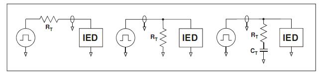
Critical lines may be either source terminated (left) or load terminated (center, right). Load terminations can be either dc (center) or ac (right). All will give similar performance so far as damping undesired ringing and overshoot, though they have different characteristics in other ways:

• Load termination can be applied to a line driving multiple IEDs along its length. Source termination distorts the waveform at the input end of the cable, and is only suitable for load(s) located at the very end of the cable. Peak current rating is:

For example, with a 5V signal and 50W termination, peak current is 100 mA.

• Source termination has the lowest power requirement, as its ac input impedance is twice the cable impedance and its dc input impedance is infinite (assuming an open circuit load). A high-drive clock output will be able to drive more source-terminated lines in parallel, than load-terminated lines. Peak current rating is:

where RT is the termination resistance and RO is the cable characteristic impedance.

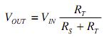
• Source termination acts as a voltage divider with the attached load. If the load impedance is low (comparable to the cable characteristic impedance), this will attenuate the signal:

For high-impedance loads, this normally is not a problem.

• AC load termination offers a combination of the advantages of the other methods. Its ac input impedance is equal to the cable impedance, but its dc input impedance is infinite (again with an infinite load). It does not act like a voltage divider with the IED load, but acts in parallel with it. Power dissipation is in between source and dc load termination. The peak current requirement, used to determine the necessary driver rating, is the same as for dc load termination.
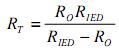
• The clock internal source termination resistor must also be accounted for in your calculations. For load termination, this will cause some attenuation of the signal:

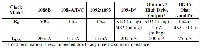
where RT is the load termination and RS is the internal termination. For source termination, you must also include the effects of the existing source impedance of the clock output – simply subtract from the desired value RT to get the external resistor value. Internal source termination values for Arbiter clocks are:

Values of Termination Components

Both source and load termination resistors should be nominally equal to the line impedance. For coaxial cables, the rated impedance is published for each cable; 50 ohms is the most common value. Twisted-pair cables are generally around 100 ohms. The exact value of the termination resistance is not critical, plus or minus 20 % generally gives acceptable results. In critical applications, it is best to experiment.

For load terminations, if the IED load resistance is less than about 10x the cable characteristic impedance, you will need to consider its effect on the termination. Generally, this allows a higher resistance value to be used:

where RT is the required termination resistance, RO is the characteristic impedance of the cable, and RIED is the IED load resistance. Since the IED input resistance is often non-linear (including an LED diode in an optocoupler), this equation gives only an approximate result and experimentation is recommended to find the optimum value RT. The equation should get you close, however.

The power rating of the resistor is normally important only for the dc load termination. The other configurations do not result in continuous power dissipation (except for high pulse rates, above 1kPPS, where the power increases with increasing frequency, up to the same value as for dc load terminations). The maximum power is from Watt’s law:

Use the next larger rated power for the resistor; for example with V=5 volts and RT=50 ohms, P is 0.5 watts; the next larger standard rating is 1 watt. For ac and source termination and signals up to 1kPPS, you can use a smaller rating such as ¼ watt.

The resistance of an ac load termination should be the same as for a dc load termination. The series capacitance CT should give a time constant 10x to 20x the electrical length of the cable, or more:

where L is cable length, v is the cable’s specified velocity factor (usually between 0.6 and 1.0), c is the speed of light (3x108 m/s), and RT is the termination resistance. The smaller the capacitance, the less the power dissipation. For a 100-ohm twisted pair (v = 0.77), 30m or 100’ long, a reasonable capacitance value is 22 nf, giving a time constant 22 nf x 100 ohms = 2.2 microseconds; which is about 17x the electrical length of 130 ns. You can test different values of capacitance to see what effect they have on your installation.

Generally, metal- or metal-oxide film resistors and monolithic ceramic capacitors represent the best value and give good results. Resistors and capacitors like this are readily available from numerous sources, including on-line vendors such as DigiKey and Mouser.

Wiring Topology – Connecting Multiple Devices to One Output

In most cases, multiple outputs can be connected to a single clock output, particularly if it is a high-drive output. Various topologies are possible. For modulated IRIG signals, choice of wiring topology is not critical.

For unmodulated IRIG (or 1PPS), in applications that require termination, a ‘star’ configuration should be used with each branch properly terminated. The total load current (again from Ohm’s law) should not exceed the rating of the output. Multiple high-impedance or ‘bridging’ loads can be connected across any load-terminated branch, but source-terminated branches should only have loads at the end. Several high-impedance loads connected within one or two meters of the end of the branch should be acceptable. You can try the specific configuration in the lab to verify that the termination works properly.

Other Digital Signals

Other digital signals such as the Programmable Pulse, 1kPPS, and IRIG Modified Manchester, may be connected following the same guidelines as for the 1PPS and IRIG-B Unmodulated signals. For the most part, the ringing and overshoot on any of these signals will be the same on the rising and falling edge, as for any other of the signals. Ringing and overshoot are determined by the rise/fall times of the signal, termination, and length and style of cable. For the signals described, ringing will have settled out well before the next transition, so you will basically be looking at the step response of the line, as terminated.

This is true so long as the electrical length of the cable (length expressed as propagation delay, typically 1 ns/ft to 1.5 ns/ft or 3 ns/m to 5 ns/m) is much less than the time between transitions. The electrical length of a 30m or 100’ cable is 150 ns, more or less; for a 1kPPS signal, the time between transitions is 500 microseconds. This is about 3000x the electrical length. For signal rates of 1MPPS and above, or much longer cable runs, this condition may no longer be true; however, the required termination for good signal fidelity is still very much the same.

Grounding Time Code Signals

From time to time, there is a discussion about how and where (and if) grounding of the timecode signal lines is required. IED designers can be tempted to use a non-isolated input in their device to save a little money. Best engineering practice generally requires any signal line to be grounded (earthed) at some point. For most analog signals, including time-code signals, this is normally the signal source.

Since ground loops are to be avoided, it is important to ground each signal at one point only. This must be the source if there is the possibility to have multiple loads attached to a given source. Therefore, time-code inputs in such a system must provide galvanic isolation.

There is also the system cost issue. Floating time-code outputs can be built, but require (costly) floating power supplies, whereas an isolated input requires no power supply. Compare a simple system having four IEDs driven by a clock: system A has one output, driving four optically-isolated IED inputs in parallel; and system B has a clock with four isolated outputs, each driving a single, grounded IED input. Clearly system A will have a lower equipment cost, since system B requires (in addition to optical isolators) floating power supplies for each independent output.

For these reasons, it has become best industry practice to ground time-code outputs from clocks, and use galvanic isolation of time code inputs to IEDs.

Fiber-Optic Distribution

No discussion of time-code distribution would be complete without mention of fiber optics. Fiber-optic cables have the advantage of immunity to electromagnetic interference. They can be used to distribute time codes in severe-EMI environments. However, while substations may reasonably be considered high-EMI environments, the expense of fiber-optic cable and drivers is generally not justified for most connections, particularly between clock and IEDs in the same rack or control room.

This is because the galvanic isolation provided at the IED input also provides great immunity to damage from substation surge voltages. The occasional transient signal propagated to the optical isolator or transformer output is easily dealt with by the pulse-conditioning or demodulation circuits in a well-designed IED, and even if a transient is detected by the countertimers, it is easily identified and ignored. As a final protection, error bypass in the local clock should guarantee continuous and accurate operation.

There are applications for fiber distribution of time codes, particularly between substations or control houses, where the length of the link makes copper connections undesirable. For these applications, where lengths can be many kilometers and losses require an ac-coupled signal, IRIG time code may be transmitted using modified Manchester encoding. This was first defined by PES-PSRC in IEEE Standard 1344-1995 (annex F) and later adopted by IRIG itself in IRIG Standard 200.

However, the cost of such systems must be weighed against the alternative of placing an additional GPS clock at the remote location. In almost all cases, the cost is lower, and reliability and flexibility greater, when a second GPS clock is used instead of a long fiber-optic link.

Delays in Distribution Wiring

The cables used to distribute IRIG-B, 1PPS and other clock outputs will delay the signals, due to the propagation time in the cable. This time is related to the speed of light, and the reduction in propagation velocity due to the dielectric constant of cable insulation being greater than 1.0. The propagation delay is:

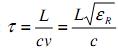where L is the length of the cable, c is the speed of light (3x108 m/s), v is the velocity factor (typically 0.6 to 1.0) and eR is the effective dielectric constant relative to vacuum, typically 1.5 to 3.

Typical delays are 1 ns/ft to 1.5 ns/ft, or 3 ns/m to 5 ns/m of cable. The same relationships hold for fiber media.

Generally, except for long cables and very-high-accuracy applications, propagation delay is a minor source of error that can be ignored.

Distributing Network Time Signals

TCP vs. UDP

To an application designer, TCP (Transport Control Protocol) with its guarantee of reliable, orderly packet delivery seems like the ideal solution to the problem of getting data from point A to point B. However, many network protocols including NTP and PTP use UDP (User Datagram Protocol) as their transport layer. UDP, like the IP layer above it, is a best-effort protocol, so lost packets and mis-ordered packets will occur. Why use UDP when TCP guarantees delivery?

The key to understanding this is that UDP places the burden of dealing with network problems on the receiving device/application layer. TCP places the burden on the sending device/transport layer. Furthermore, many devices in a power-system network are microcontroller-based, and have limited memory for data buffers.

In a real-time, substation environment, placing this burden on the sending device often results in data backups, lost packets, and under certain conditions, stack lockup. The magnitude of this problem depends on a complex interaction of the data rate, channel reliability (Bit Error Rate), and size of available buffers. Note that these problems (discarded packets, in particular) are exactly what the software designer is trying to avoid by using TCP in the first place.

In real-time applications, UDP therefore favors overall reliability of the connection, keeping data flowing at the cost of occasional lost packets. TCP favors the reliability of a single data packet over connection reliability. TCP will sometimes ‘throw itself on the funeral pyre’ trying to get that lost packet through. Note that in non-real-time applications (file transfers, email, web surfing) stack reliability is not so big an issue, since data flows can be suspended while the retry is attempted. In real time, the incoming data backs up, with nowhere else to go.

So, if the goal is to maximize overall system reliability when dealing with the limited resources sometimes encountered in substation IEDs, UDP is a superior choice. While there will be occasional lost packets, the overall system will be more reliable. Given the choice of a lost packet or a failed connection, which would you choose?

Managed Switch Configuration

Managed switches provide the ability to prioritize network traffic, to classify it into different flows, to protect certain devices from access (or data overload) by other devices, and many other features which can (and we believe, must) be used to ensure reliable and orderly operation of substation networks. Few substation engineers are familiar with this issue.

For the most part, network infrastructure is treated like a ‘black box’ – it is plugged in, turned on, and if it seems to work everything must be OK. This approach comes down in many cases from the IT department. Familiar with the needs of enterprise networking, they are not familiar with the real-time, mission-critical needs of power system protection and control.

Problems with reliable operation of Phasor Measurement Unit data systems, and problems with achieving accurate synchronization using network timing methods such as NTP, are beginning to show the need for proper management of the substation communications infrastructure. These two applications – PMUs and NTP – are in many cases the first real-time applications for substation networking, where the network is being asked to do more than download an occasional configuration or data file. As the new IEC 61850 standard begins to be used more widely, these problems will become more widespread.

Managed switches provide features like these to help ensure reliable operation of missioncritical applications:

• QoS or quality of service. This is the ability of a switch to classify traffic and assign different priority to different types of data. Packets may be classified on the basis of things like: source and destination logical (L4) ports or IP addresses; ToS/DS field in IP header; VLAN membership; physical port; MAC address; and others, including the value of any specified octet in the header(s).
• VLAN. Virtual LAN is grouping of the physical ports on the switch into one or more groups, which the switch treats as logically separate networks. Devices on separate VLANs, though connected to the same switch, cannot see each other. Some devices can be members of more than one VLAN. VLANs can be port-based or based on tags (IEEE 802.1Q) or protocol (802.1v). VLANs can be used to isolate traffic, including broadcast and multicast traffic, from different devices and also to provide security.
• Hardware port configuration. Features like rate (10/100), full or half duplex, and Auto-MDIX reconfiguration can be set. Ports can be set to a fixed MAC address, so that if a device is unplugged and another connected in its place, communication is impossible. These features can be used to improve reliability (auto-negotiation sometimes fails in noisy environments) and security.
• IGMP snooping. Ethernet traffic comes in three varieties: directed frames (sent to a single device); broadcast frames (sent to all devices), and multicast frames (sent to a group of devices). IGMP (Internet Group Multicast Protocol) Snooping allows the switch to send multicast traffic only to devices that have requested it. Since an overload of incoming traffic can cause problems for a receiving device, particularly IEDs with simple microcontrollers, this feature helps to enhance reliability.
• Filtering. The switch can filter traffic to a port based on many of the same classification rules used for QoS and VLAN control. For example, a port could be set to forward only frames addressed directly to the specified MAC address. This would stop port overload caused by broadcast or multicast traffic.
• SLA/Traffic Management. SLA (Service Level Agreement) and other traffic management rules can be set, reserving a certain portion of bandwidth for specified classes of traffic. This allows priority messages – SNTP messages or IEC 61850 GOOSE messages, for example – to enjoy higher-priority, guaranteed reservations, even when the network is busy with a high level of background traffic. Without these rules, all traffic has the same priority, and important or time-critical messages can get lost in the crowd.
• SNMP Support. Simple Network Management Protocol (SNMP) provides a standardized means to control and monitor switch and router performance, based on a standardized Management Information Block (MIB) which describes the switch capabilities.
• Port or Traffic Mirroring. Switches, unlike hubs, send packets only to those device(s) which are the intended recipients. Analyzing network traffic can be simplified if the switch provides the capability to ‘mirror’ traffic to another port, allowing you to connect a protocol analyzer such as WireShark.

PES-PSRC has convened a working group (H2) to address the configuration of Ethernet devices for critical substation applications.

Controlling Message Traffic Priority

To establish rules setting priority, two things must be done. First, the protection engineer, or substation communications engineer, must analyze the expected traffic flows and categorize them into classes. This categorization must be based on identifiable parameters that are a part of the message structure, or can be made a part of the message structure by proper IED configuration (note that few IEDs provide tools to customize this at this time). These must be parameters that a managed switch can identify, and use to classify and prioritize traffic.

Then, a switch that can support the required packet classification should be selected and installed. The switch must be programmed with the ruleset, and its performance tested and verified (again, few tools exist now to help with this, though packet analyzers such as WireShark can help).

Unsolicited Broadcast and Multicast Traffic

We have seen several problems where IEDs operate fine until XYZ device is turned on; or work for a while and then stop; or otherwise misbehave. Often, re-configuring the network, moving the IED away from some other device, fixes the problem. So far, in most cases the culprit has been found (or suspected) to be unsolicited broadcast or multicast traffic, put on the network by another application.

Filtering in the switch is a powerful tool to prevent overload from unsolicited traffic. Managed switches usually provide several methods to control broadcast and multicast traffic, including IGMP snooping and MAC-based filtering.

Other Network Traffic

Even desired network traffic can cause problems. During a major event, every engineer on duty is likely to be on-line, downloading files and trying to develop an understanding of the unfolding events. This spike in network traffic can cause failures due to data overload in a network that had previously been running without incident.

Naturally, this is a bad time to find out that the switch configuration does not provide proper priority and protection for mission-critical real-time traffic. Managed switches should be configured to protect this traffic, and tests performed (using simulators and protocol analyzers, for example) to verify that delivery of essential message traffic continues even during an onslaught of unexpected background traffic.

(S)NTP, PTP, and PMU Port Information

SNTP and NTP message traffic uses UDP port 123 (base 10). PTP (IEEE-1588) uses ports 319 (for time-tagged messages) and 320 (for other messages). PTP is normally implemented with UDP, though TCP is also supported.

Phasor measurement units (PMUs) use TCP port 4712 and UDP port 4713, though this is not a fixed assignment. The Arbiter 1133A PMU also uses TCP port 4714 to control its 2nd logical PMU function.

Specific PTP Requirements for the Network

As described earlier, PTP comes in two varieties: software-only, and hardware-aided. Software-only implementations can run on any typical network, and will deliver performance similar to SNTP in these applications.

Hardware-aided implementations can provide accuracy of 20 ns to 100 ns, but all components handling PTP message traffic must support the hardware-aided configuration. These include:

• PTP Grandmaster. This is a clock with a source of traceable, accurate time (typically GPS but it could receive, for example, IRIG time from another GPS clock). It acts as a master or server on the PTP network. One is required, though PTP describes methods for more than one to exist on a network, with a ‘best master clock’ algorithm to allow the network to choose which to use at any point in time.
• PTP Client(s). This is a device such as an IED that accepts time from a grandmaster. It does not synchronize any other device using PTP, though it could generate time code outputs like 1PPS or IRIG-B.
• PTP Switches. These come in two varieties: switch with a boundary clock; and a transparent switch. Both of these are required not to forward PTP frames, but to handle them according to specific rules defined in the standard.
  A switch with boundary clock has an internal clock that is synchronized to a grandmaster, and in turn synchronizes clients connected to it. It creates a separate ‘domain’ in that its master is not aware of traffic directed to it. It responds to requests for synchronization as the master clock of its domain.
  A transparent switch does not operate an internal clock, but instead forwards PTP messages with modification. The time tags in the PTP messages are adjusted, based on the time the packet is stored before it can be forwarded. A transparent switch does not create a new domain, and the grandmaster receives and responds to every synchronization request sent by the clients.

« Back to Advancing the Technology Index